Scalar potential

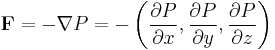
A scalar potential is a fundamental concept in vector analysis and physics (the adjective scalar is frequently omitted if there is no danger of confusion with vector potential). The scalar potential is an example of a scalar field. Given a vector field F, the scalar potential P is defined such that:

$\mathbf{F} = -\nabla P = - \left( \frac{\partial P}{\partial x}, \frac{\partial P}{\partial y}, \frac{\partial P}{\partial z} \right)$ ,^[1]

where ∇P is the gradient of P and the second part of the equation is minus the gradient for a function of the Cartesian coordinates x,y,z.^[2] In some cases, mathematicians may use a positive sign in front of the gradient to define the potential.^[3] Because of this definition of P in terms of the gradient, the direction of F at any point is the direction of the steepest decrease of P at that point, its magnitude is the rate of that decrease per unit length.

In order for F to be described in terms of a scalar potential only, the following have to be true:

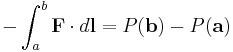$-\int_a^b \mathbf{F}\cdot d\mathbf{l} = P(\mathbf{b})-P(\mathbf{a})$ , where the integration is over a Jordan arc passing from location a to location b and P(b) is P evaluated at location b .
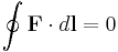$\oint \mathbf{F}\cdot d\mathbf{l}=0$ , where the integral is over any simple closed path, otherwise known as a Jordan curve.
${\nabla}\times{\mathbf{F}} =0$

The first of these conditions represents the fundamental theorem of the gradient and is true for any vector field that is a gradient of a differentiable single valued scalar field P. The second condition is a requirement of F so that it can be expressed as the gradient of a scalar function. The third condition re-expresses the second condition in terms of the curl of F using the fundamental theorem of the curl. A vector field F that satisfies these conditions is said to be irrotational (Conservative).

Scalar potentials play a prominent role in many areas of physics and engineering. The gravity potential is the scalar potential associated with the gravity per unit mass, i.e., the acceleration due to the field, as a function of position. The gravity potential is the gravitational potential energy per unit mass. In electrostatics the electric potential is the scalar potential associated with the electric field, i.e., with the electrostatic force per unit charge. The electric potential is in this case the electrostatic potential energy per unit charge. In fluid dynamics, irrotational lamellar fields have a scalar potential only in the special case when it is a Laplacian field. Certain aspects of the nuclear force can be described by a Yukawa potential. The potential play a prominent role in the Lagrangian and Hamiltonian formulations of classical mechanics. Further, the scalar potential is the fundamental quantity in quantum mechanics.

Not every vector field has a scalar potential. Those that do are called conservative, corresponding to the notion of conservative force in physics. Examples of non-conservative forces include frictional forces, magnetic forces, and in fluid mechanics a solenoidal field velocity field. By the Helmholtz decomposition theorem however, all vector fields can be describable in terms of a scalar potential and corresponding vector potential. In electrodynamics the electromagnetic scalar and vector potentials are known together as the electromagnetic four-potential.

1 Integrability conditions
2 Altitude as gravitational potential energy
3 Pressure as buoyant potential
4 Calculating the scalar potential
5 See also
6 References

Integrability conditions

If F is a conservative vector field (also called irrotational, curl-free, or potential), and its components have continuous partial derivatives, the potential of F with respect to a reference point $\mathbf r_0$ is defined in terms of the line integral:

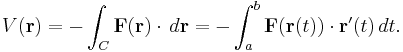
$V(\mathbf r) = -\int_C \mathbf{F}(\mathbf{r})\cdot\,d\mathbf{r} = -\int_a^b \mathbf{F}(\mathbf{r}(t))\cdot\mathbf{r}'(t)\,dt.$

where C is a parametrized path from $\mathbf r_0$ to $\mathbf r,$

$\mathbf{r}(t), a\leq t\leq b, \mathbf{r}(a)=\mathbf{r_0}, \mathbf{r}(b)=\mathbf{r}.$

The fact that the line integral depends on the path C only through its terminal points $\mathbf r_0$ and $\mathbf r$ is, in essence, the path independence property of a conservative vector field. The fundamental theorem of calculus for line integrals implies that if V is defined in this way, then $\mathbf{F}= -\nabla V,$ so that V is a scalar potential of the conservative vector field F. Scalar potential is not determined by the vector field alone: indeed, the gradient of a function is unaffected if a constant is added to it. If V is defined in terms of the line integral, the ambiguity of V reflects the freedom in the choice of the reference point $\mathbf r_0.$

Altitude as gravitational potential energy

An example is the (nearly) uniform gravitational field near the Earth's surface. It has a potential energy

$U = m g h$

where U is the gravitational potential energy and h is the height above the surface. This means that gravitational potential energy on a contour map is proportional to altitude. On a contour map, the two-dimensional negative gradient of the altitude is a two-dimensional vector field, whose vectors are always perpendicular to the contours and also perpendicular to the direction of gravity. But on the hilly region represented by the contour map, the three-dimensional negative gradient of U always points straight downwards in the direction of gravity; F. However, a ball rolling down a hill cannot move directly downwards due to the normal force of the hill's surface, which cancels out the component of gravity perpendicular to the hill's surface. The component of gravity that remains to move the ball is parallel to the surface:

$F_S = - m g \ \sin \theta$

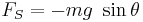
where θ is the angle of inclination, and the component of F_S perpendicular to gravity is

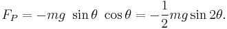
$F_P = - m g \ \sin \theta \ \cos \theta = - {1 \over 2} m g \sin 2 \theta.$

This force F_P, parallel to the ground, is greatest when θ is 45 degrees.

Let Δh be the uniform interval of altitude between contours on the contour map, and let Δx be the distance between two contours. Then

$\theta = \tan^{-1}{\Delta h \over \Delta x}$

so that

$F_P = - m g { \Delta x \, \Delta h \over \Delta x^2 %2B \Delta h^2 }.$

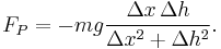
However, on a contour map, the gradient is inversely proportional to Δx, which is not similar to force F_P: altitude on a contour map is not exactly a two-dimensional potential field. The magnitudes of forces are different, but the directions of the forces are the same on a contour map as well as on the hilly region of the Earth's surface represented by the contour map.

Pressure as buoyant potential

In fluid mechanics, a fluid in equilibrium, but in the presence of a uniform gravitational field is permeated by a uniform buoyant force that cancels out the gravitational force: that is how the fluid maintains its equilibrium. This buoyant force is the negative gradient of pressure:

$\mathbf{f_B} = - \nabla p. \,$

Since buoyant force points upwards, in the direction opposite to gravity, then pressure in the fluid increases downwards. Pressure in a static body of water increases proportionally to the depth below the surface of the water. The surfaces of constant pressure are planes parallel to the ground. The surface of the water can be characterized as a plane with zero pressure.

If the liquid has a vertical vortex (whose axis of rotation is perpendicular to the ground), then the vortex causes a depression in the pressure field. The surfaces of constant pressure are parallel to the ground far away from the vortex, but near and inside the vortex the surfaces of constant pressure are pulled downwards, closer to the ground. This also happens to the surface of zero pressure. Therefore, inside the vortex, the top surface of the liquid is pulled downwards into a depression, or even into a tube (a solenoid).

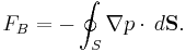
The buoyant force due to a fluid on a solid object immersed and surrounded by that fluid can be obtained by integrating the negative pressure gradient along the surface of the object:

$F_B = - \oint_S \nabla p \cdot \, d\mathbf{S}.$

A moving airplane wing makes the air pressure above it decrease relative to the air pressure below it. This creates enough buoyant force to counteract gravity.

Calculating the scalar potential

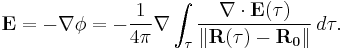
Given a vector field E, its scalar potential Φ can be calculated to be

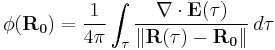
$\phi(\mathbf{R_0}) = {1 \over 4 \pi} \int_\tau {\nabla \cdot \mathbf{E}(\tau) \over \| \mathbf{R}(\tau) - \mathbf{R_0} \|} \, d\tau$

where τ is volume. Then, if E is irrotational (Conservative),

$\mathbf{E} = -\nabla \phi = - {1 \over 4 \pi} \nabla \int_\tau {\nabla \cdot \mathbf{E}(\tau) \over \| \mathbf{R}(\tau) - \mathbf{R_0} \|} \, d\tau.$

This formula is known to be correct if E is continuous and vanishes asymptotically to zero towards infinity, decaying faster than 1/r and if the divergence of E likewise vanishes towards infinity, decaying faster than 1/r².

References

^ Herbert Goldstein. Classical Mechanics (2 ed.). pp. 3–4. ISBN 9780201029185.
^ The second part of this equation is ONLY valid for Cartesian coordinates, other coordinate systems such as cylindrical or spherical coordinates will have more complicated representations. derived from the fundamental theorem of the gradient.
^ See [1] for an example where the potential is defined without a negative. Other references such as Louis Leithold, The Calculus with Analytic Geometry (5 ed.), p. 1199 avoid using the term potential when solving for a function from its gradient.